Ai Pengya

Independent t-test is also called two sample t-test. It is aimed at comparing the means of two groups. For example, I want to compare whether the average mean of environmental knowledge is the same between males and females. Academically, we often propose alternative hypothesis like “environmental knowledge is different between males and females.” While statistically, the null hypothesis we will test is “the average environmental knowledge is the same between males and females.”

The logic is that if we reject the null hypothesis (p<.05), then it is highly likely that the alternative hypothesis (two means are different) is true in the population.

Independent t-test

I’m continuing using the sample data

The mean of females is 3.8663, males 4.5879 (you can first select cases and calculate the means separately, but here I just use the reports from the independent t-test). Looks like the knowledge of males is much higher than females. However, as stated in the one sample t-test, such a difference is only detected by this specific sample. We need to get the p-value to see how likely the difference exists in the population.

(One might have questions about how we can determine this. The key point is the standard error. If the error is toooo high, it means that even the sample mean is different, but it might be highly due to the error. Take one sample t-test as an example, 4.24 is different from 5. But if I got a very high error from my sample. Then the results may tell me that such a difference might just be because of the error. The population mean is likely to be 5 or 3 or any values within a very large range. However, if I get a very small error from the sample, then it means that if I get another sample from the population, the mean will not have many deviations from what I get now (but you can always say there could be very large differences. It is just a game of probability). Therefore, I’m more confident to say 4.24 is the population mean and the 5 or 3 is highly likely not the population mean.)

In SPSS, the independent t-test is in Analyze -> Compare Means -> Independent-samples T-Test

Enter the variable you want to test in test variables, and the grouping variable in grouping variable. Here, gender is the group. What is the group variable is subject to the question you have. For example, in experiments, the grouping variable might be the manipulation.

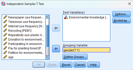
I coded female as 0 and male as 1 in the gender variable. Therefore, I click “Define Groups” and enter 0 and 1 and Continue. Then click “OK” and get the results.

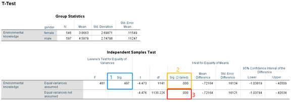
Then you may be confused by the three p-values here, one is non-significant (>0.05), but the other two are significant (<0.05). This is one of the questions I often got from students when I taught them. If you don’t want to know the reason, I would recommend only looking at the third p-value, which is the one in the second row, because it is the safest.

The easiest way to calculate the t statistics requires the variances to be the same between the two groups. This is very different from one-sample t-test as in one-sample t-test, there is only one thing changing. The number/constant you choose to compare is not a variable because it cannot change. However, in independent t-test, there are two variables: one from the 1st group and the other from the 2nd group. It is possible that the variance in one group is very high, but the variance of the other is pretty low. In this case (different variances), the original way to calculate the p-value is not appropriate. But in some cases, the variances could be “same” between the two groups. Then we can use the original formula.

Therefore, we need first to examine whether the variances are the same between the two groups, which is the use of the first p-value. The null hypothesis of the first p-value is that the variances are the same among two groups, which is examined with F test. So we got a p-value of 0.497, larger than 0.05. This means that we don’t have enough evidence to say that the variances are different between the two groups. Therefore, we can look at the p-value (the 2nd p-value) in the first row (Equal variances assumed), which is less than 0.001. This means that based on this sample, the environmental knowledge of females is unlikely to be the same of males. In other words, the results supported our hypothesis that “environmental knowledge is different between males and females.”

Alternatively, if the first Sig. of the F test is significant (p-value < 0.05), we can only look at the second row (Equal variances not assumed, the 3rd p-value) because you reject the hypothesis that the variances are the same between two groups (cannot assume the variances are equal anymore). But luckily, the p-value is very large in the example. And also, in my understanding, there is no harm in always looking at the row that does not assume equal variances because you can always say, it is possible that the variances are different.

Anyway, according to the 2nd p-value, we can conclude that the environmental knowledge of females is statistically significantly different from males (p<.001). You can look for journals in specific fields to see the common reporting styles and what statistics should be reported.