Linear regression is widely used to assess the relationships between multiple variables. We usually use linear regression for two reasons: (1) Linear relationship is easier to interpret; (2) Many non-linear relationships can be expressed in linear format ¹.

A linear regression model has one dependent variable and usually contains more than one independent variable. Mathematically, it can be expressed as . Here, I wish to emphasize the difference between a regression model and zero-order linear correlation (e.g., Pearson correlation coefficient). Zero-order linear correlation means the correlation between two variables without partial out other variables’ effects. By contrast, the results of linear regression show the relationship between one independent variable (e.g., ) and dependent variable (), being partialled out other variables’ relationship with $y$ (if we treat as the interested variable, then other variables include to here). These other variables are usually called control variables or covariates ².

For example, we are interested in the relationship between media use frequency and environmental knowledge. We use media use frequency (independent variable) to predict environmental knowledge (dependent variable). If we use correlation or simple regression (one independent variable, one dependent variable), we are studying the correlation between the two variables. But we know that some other factors, such as age and gender, may simultaneously influence media use frequency and environmental knowledge. If we want to see the pure effect³ of media use on environmental knowledge, we need to add gender and education as control variable to partial out the effects of gender and education on environmental knowledge.

There are many ways to estimate such a model. Usually we use Ordinary Least Square (OLS) to estimate a linear regression model. The main idea of OLS is to minimize the sum of the square of the differences between the observed value and the predicted value. For example, in the figure below, the way to estimate the regression function is to minimize the square of the distances.
{% asset_img Fig1.png Regression %}
(Note. This figure shows the case of simple regression. For multiple regression, it needs to be estimated with matrix, and it cannot be shown with a 2D plot)

OLS has many advantages. If the data satisfied the assumptions in Gauss–Markov theorem, then the OLS estimator is the best linear unbiased estimator (BLUE). But this is very complex, talking about the details can take a whole semester. But I note them here because sometimes people could have concerns over the results of OLS because of these assumptions. For example, if there is exogeneity problem, then the validity of the coefficient is questionable.

SPSS example:

Sample data download ⁴
The example is to estimate the relationship between media use frequency and environmental knowledge level (both are seen as continuous variable).

Zero-order correlation

SPSS steps:

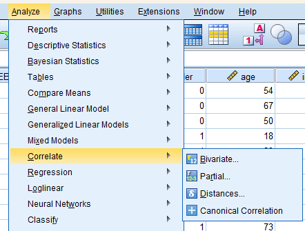
1. Analyze -> Correlate -> Bivariate
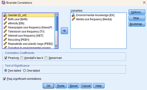
2. Add the two interested variables (i.e., media and environemtnal knowledge in this case)
3. Click “OK” and get the results

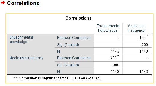
Interpretation: Environmental knowledge is significantly positively correlated with media use frequency (). Or media use frequency is significantly positively correlated with environmental knowledge ().
(Note. For professional report, please find published articles in specific field)

Simple regression (no control variable)

1. Analyze -> Regression -> Linear
2. Use environmental knowledge as dependent variable and media use frequency as independent variable.
3. Click “OK” then we can get:

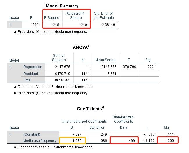
Interpretation: The most important things to look at/report are 1) (standard or unstandardized) coefficient (positive or negative); 2) p-value (Sig., usually <.05 is seen as significant); model fit (R-square/Adj R-square)

In the example, the results show that media use has significant positive relationship with individuals’ environmental knowledge (). (Note. For professional report, please find published articles in specific field)

You can find that the R value and standardized coefficient are actually the same as the Pearson correlation coefficient. It is not a coincidence. They should be the same as they both are estimating the linear relationship between two variables without controlling anything else. It can be mathematically proven, but I will not show it here.

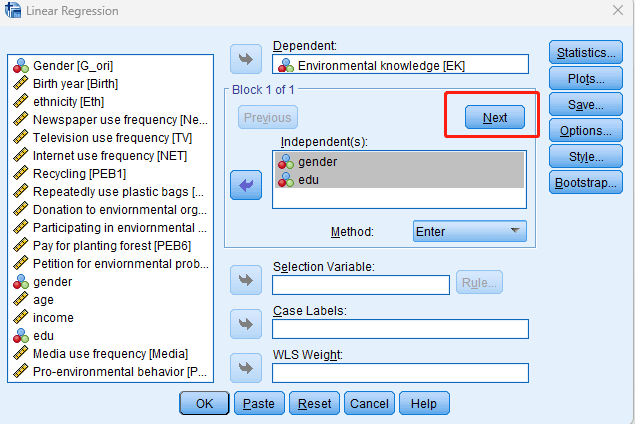
Multiple regression (with gender and education as control variable)

1. Same as simple regression.
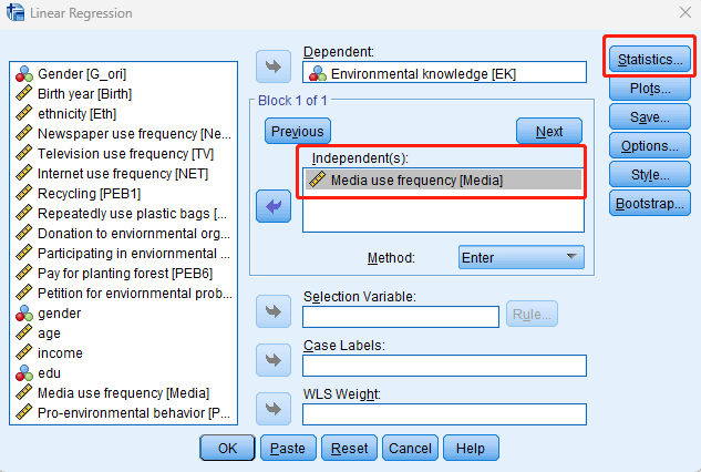
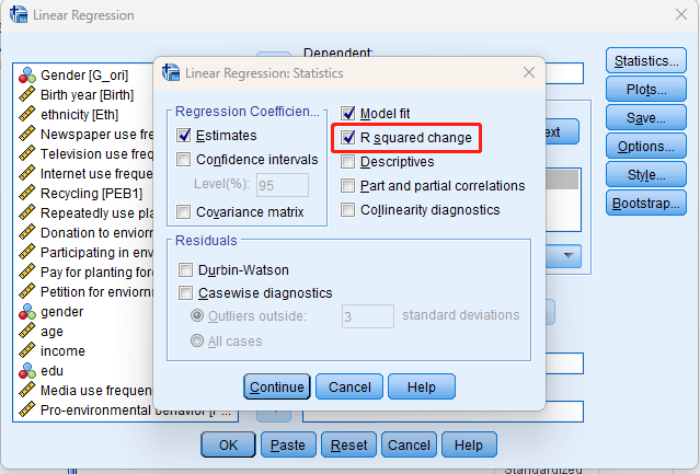
2. For multiple regression, sometimes we wish to estimate how adding the interested variables changes the model fit. Therefore, we may add the control variables and interested variables in different blocks. Here, I add gender and education in the first block, and media use in the second block. In “Statistics”, I clicked the “R-square change” to see how much R-square changes (and whether the change is significant or not) after adding media use to the model which has only gender and education as predictors.
3. Click “Continue” and “OK”, then we can see the results

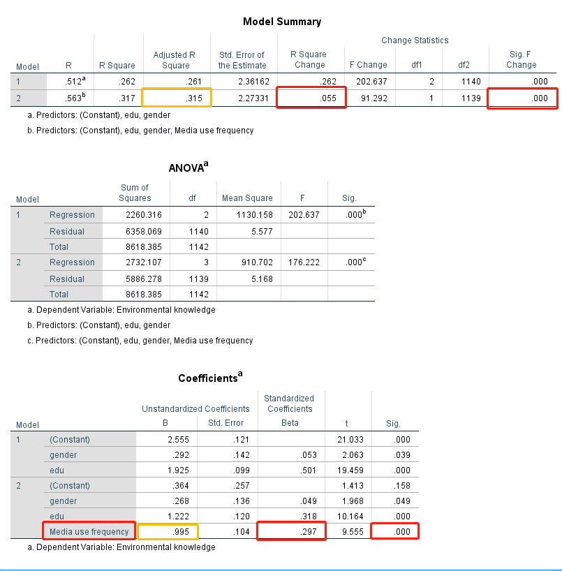
Interpretation:

• After controlling gender and education, media use positively predict environmental knowledge (). (We can see that the standardized coefficient decreased a bit, it shows that some effects are partialled out by gender and education. But it is very hard to explain how adding control variables changes the results. Anyway, it shows the results are different.)
• Adding media use significantly improves the model fit ().

(Note. For professional report, please find published articles in specific field)